Empirical estimation of FDR

A brief introduction to the theory of local and global False Discovery Rates

Introduction

A more detailed explanation is given in a my previous post Background of two groups model.

An idea I put into package CRISPhieRmix (R package, paper) is a way to estimate global false discovery rates (FDRs) from local fdrs when it is too difficult to directly compute the global FDR.

The global FDR is the expected fraction of false discoveries among the ones that we call significant. The way we usually think about this is that we’re gonna compute some one dimensional statistic (e.g. \(p\)-value or \(z\)-value) for tests/categories/hypotheses \(i = 1, \ldots, n\), we’re gonna set a threshold \(p^{*}\) (or \(z^{*}\) if we look in terms of a \(z\)-value), then we’re gonna call as significant those with \(p_{i} < p^{*}\) (or \(| z_{i} | > z^{*}\)). Then the expected fraction of false discoveries among the set that we called significant is the global FDR, or \[ \mathrm{E} \left( \sum_{i = 1}^{n} 1 \left( \text{test } i \text{ is null} \cap p_{i} < p^{*} \right) / \sum_{i=1}^{n} 1 \left(p_{i} < p^{*} \right) \right). \] Note that there is some difficulty in defining the FDR when no tests are called significant. To get around this difficulty we can define marginal FDR (mFDR) as the ratio of the expected number of nulls called significant divided by the expected number of tests called significant, with the understanding that \(0/0 = 0\) (see Storey, 2010). I.e. \[ \text{mFDR} = \frac{\mathrm{E} \big( \sum_{i = 1}^{n} 1 \left( \text{test } i \text{ is null} \cap p_{i} < p^{*} \right) \big)}{\mathrm{E} \big( \sum_{i = 1}^{n} 1(p_{i} < p^{*}) \big)}. \]

Similarly, the local fdr (following Efron’s notation of keeping the local fdr in lower case) is the expected probability that an individual test is false. So for example, for test \(i\) we get \(p\)-value \(p_{i}\) then the local fdr is \[ \Pr(\text{test } i \text{ is null} | p_{i}). \]

Empirical estimation of the global FDR

The idea for empirical estimation came from an anology from Efron, 2005, the local false discovery rate is akin to the pdf and the global FDR is akin the cdf. We can see this from the (rather loose) definitions given above. Indeed, formally the global false discovery rates can be defined as the integral over the tail area of the local false discovery rates, as well as the intuition that the overall (global) FDR at a given threshold must be equal to the average of the individual local FDRs that are called significant at the threshold.

This intuition leads directly to the an easy way to estimate the global FDRs when we have the local fdrs, we just take the average of all local fdr’s lower than the one under consideration to be the estimate of the global FDR. In fact, this is an unbiased estimate of the marginal false discovery rate.

We’ll show this in the 1-dimensional case. For a measurement \(x\), we assume that the measurements follow a mixture distribution with \(x \sim f = (1- p) f_{0} + p f_{1}\). \(p\) is the probability that a randomly selected test will be non-null, \(f_{0}\) is the distribution of null cases, and \(f_{1}\) is the distribution of non-null cases. \[ \begin{aligned} \text{mFDR}(x) &\approx \frac{\mathrm{E} \big( \sum_{i = 1}^{n} 1(x_{i} \geq x \cap \text{ test } i \text{ is null}) \big)}{\mathrm{E} \big( \sum_{i = 1}^{n} 1(x_{i} \geq x) \big)} \notag \\ &= \frac{\int_{|z| \geq x} (1 - p) f_{0} (z) dz }{\int_{|z| > x} f(z) dz} \notag \\ &= \frac{\int_{|z| \geq x} \frac{(1 - p) f_{0} (z)}{f(z)} f(z) dz}{\int_{|z| \geq x} f(z) dz} . \notag \\ & = \frac{\mathrm{E} \big(\text{fdr}(z) \cdot 1(|z| \geq x) \big)}{\mathrm{E} \big( 1(|z| \geq x) \big)} \notag \\ &\approx \frac{\frac{1}{N} \sum_{i = 1}^{n} \text{fdr}(x_{i}) 1 (\text{fdr}(x_{i}) \leq \text{fdr}(x))}{\frac{1}{N} \sum_{i = 1}^{n} 1 (\text{fdr}(x_{i}) \leq \text{fdr}(x))}. \notag \\ & \notag \end{aligned} \]

The advantage for this method is that in some cases the local FDR is easy to compute but the global FDR is difficult. Such I case I encountered in my hierarchical mixture modeling of pooled CRISPR screens. Computing the global FDRs here involves integration over the level sets of a mixture model, which can be difficult. Below is an example of the level sets for when we have 2 guides (measurements) per gene, more guides makes it even more complicated. [levelSets2D.png]

Simulations

1-D case

The simplest case is the one dimensional case. We’ll assume that we have a normal mixture model, \[ f(x) \sim (1 - p) \mathcal{N}(0, \sigma_{0}^2) + p \mathcal{N}(\mu, \sigma_{1}^{2}). \] We’ll compare two cases, fitting the mixture model and computing the local FDR and global FDR from the empirical method, and the exact method (because it’s easy to compute in this case).

set.seed(12345)
mu0 = 0
mu1 = 3
sigma0 = 1
sigma1 = 1
p = 0.95
N = 10000
labels = rbinom(N, prob = 1 - p, 1)
mu_vec = sapply(labels, function(i) if(i == 1) mu1 else mu0)
sigma_vec = sapply(labels, function(i) if(i == 1) sigma1 else sigma0)
# sanity check
stopifnot(sum(mu_vec != 0)/length(mu_vec) == sum(labels)/length(labels))
x = rnorm(N, mean = mu_vec, sd = sigma_vec)

mixfit = mixtools::normalmixEM2comp(x, lambda = c(0.5, 0.5), 
                                    mu = c(0, 1), sigsqrd = c(1, 1))

## number of iterations= 1000

print("fitted proportions: ")

## [1] "fitted proportions: "

print(mixfit$lambda)

## [1] 0.94405034 0.05594966

print("fitted means: ")

## [1] "fitted means: "

print(mixfit$mu)

## [1] -0.008031135  2.656248538

print("fitted sd's: ")

## [1] "fitted sd's: "

print(mixfit$sigma)

## [1] 0.9948498 1.1280971

# taken from https://tinyheero.github.io/2015/10/13/mixture-model.html
plot_mix_comps <- function(x, mu, sigma, lam) {
  lam * dnorm(x, mu, sigma)
}
library(ggplot2)
ggplot(data.frame(x = x) ) +
  geom_histogram(aes(x, ..density..), binwidth = 1, colour = "black", 
                 fill = "white") +
  stat_function(geom = "line", fun = plot_mix_comps,
                args = list(mixfit$mu[1], mixfit$sigma[1], lam = mixfit$lambda[1]),
                colour = "red", lwd = 1.5) +
  stat_function(geom = "line", fun = plot_mix_comps,
                args = list(mixfit$mu[2], mixfit$sigma[2], lam = mixfit$lambda[2]),
                colour = "blue", lwd = 1.5) +
  ylab("Density") + theme_bw()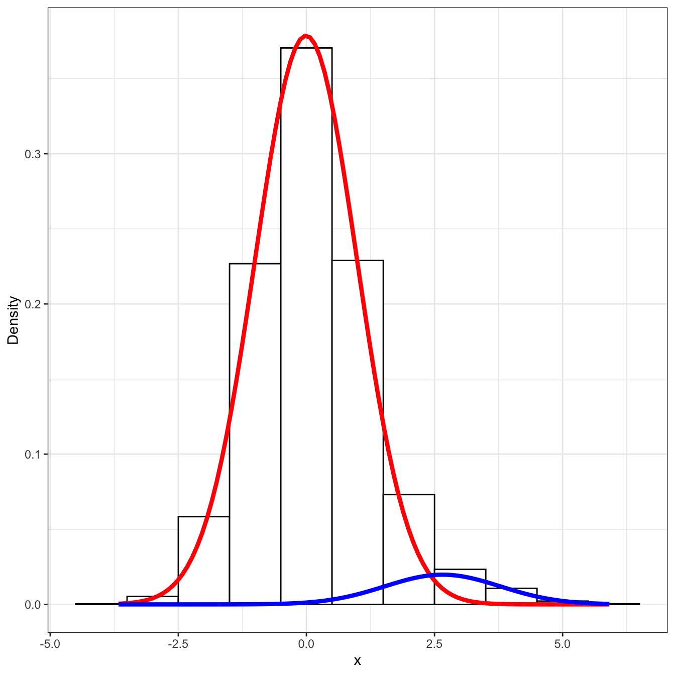

The local FDR here is easy to compute, \[ \Pr(i \text{ is null} | x_{i}) = \frac{p f_{1} (x_{i} | \mu_{1}, \sigma_{1})}{(1 - p) f_{0}(x_{i} | \mu_{0}, \sigma_{0}) + p f_{1} (x_{i} | \mu_{1}, \sigma_{1})}. \] Similarly the global mFDR is equal to \[ mFDR(i) = \frac{\int_{x \geq x_{i}} p f_{1} (x | \mu_{1}, \sigma_{1}) dx}{\int_{x \geq x_{i}} (1 - p) f_{0}(x | \mu_{0}, \sigma_{0}) + p f_{1} (x | \mu_{1}, \sigma_{1}) dx}. \] Of course, the global FDR (not marginal) has the integral outside the fraction above, but the above equation is much easier to compute because the integrals can be calculated from the cdf of the normal distribution.

normal_2group_loc_fdr <- function(x, p, mu, sigma){
  # the assumption here is that the null group is the second group
  stopifnot((length(p) == length(mu)) &
            (length(mu) == length(sigma)) &
            (length(sigma) == 2))
  p0 = p[1]*dnorm(x, mu[1], sigma[1])
  p1 = p[2]*dnorm(x, mu[2], sigma[2])
  return(p1/(p0 + p1))
}

normal_2group_mFDR <- function(x, p, mu, sigma){
  # the assumption here is that the null group is the second group
  stopifnot((length(p) == length(mu)) &
            (length(mu) == length(sigma)) &
            (length(sigma) == 2))
  p0 = p[1]*pnorm(x, mu[1], sigma[1], lower.tail = FALSE)
  p1 = p[2]*pnorm(x, mu[2], sigma[2], lower.tail = FALSE)
  return(p0/(p0 + p1))
}

Now let’s compare the methods. For comparison we will also include the standard Benjamini-Hochberg correct p-value method of computing FDRs.

BH_FDR <- function(x, mu0, sigma0){
  pvals = sapply(x, function(y) pnorm(y, mu0, sigma0, lower.tail = FALSE))
  return(p.adjust(pvals, method = "BH"))
}

compare_fdr <- function(x, p, mu, sigma, labels){
  loc_fdr = sapply(x, function(y) normal_2group_loc_fdr(y, p, mu, sigma))
  loc_mFDR = sapply(x, function(y) mean(loc_fdr[which(x >= y)]))
  mFDR = sapply(x, function(y) normal_2group_mFDR(y, p, mu, sigma))
  bh = BH_FDR(x, mu[1], sigma[1])
  true_fdr = sapply(1:length(x), function(i) sum(labels[which(x >= x[i])] == 0)/length(which(x >= x[i])))
  return(data.frame(x = x,
                    loc_fdr = loc_fdr,
                    loc_mFDR = 1 - loc_mFDR,
                    mFDR = mFDR,
                    BH_FDR = bh,
                    true_FDR = true_fdr))
}

normal_2_group_fdr_comparison = compare_fdr(x, mixfit$lambda, mixfit$mu, mixfit$sigma, labels)

df = data.frame(estimated_fdr = c(normal_2_group_fdr_comparison$loc_mFDR, 
                                  normal_2_group_fdr_comparison$mFDR, 
                                  normal_2_group_fdr_comparison$BH_FDR), 
                method = rep(c("loc_mFDR", "mFDR", "BH"), each = N),
                true_fdr = rep(normal_2_group_fdr_comparison$true_FDR, times = 3))
ggplot(df, aes(y = true_fdr, x = estimated_fdr, col = method)) + geom_line() + scale_colour_brewer(palette = "Set1") + theme_bw() + geom_abline(intercept = 0, slope = 1)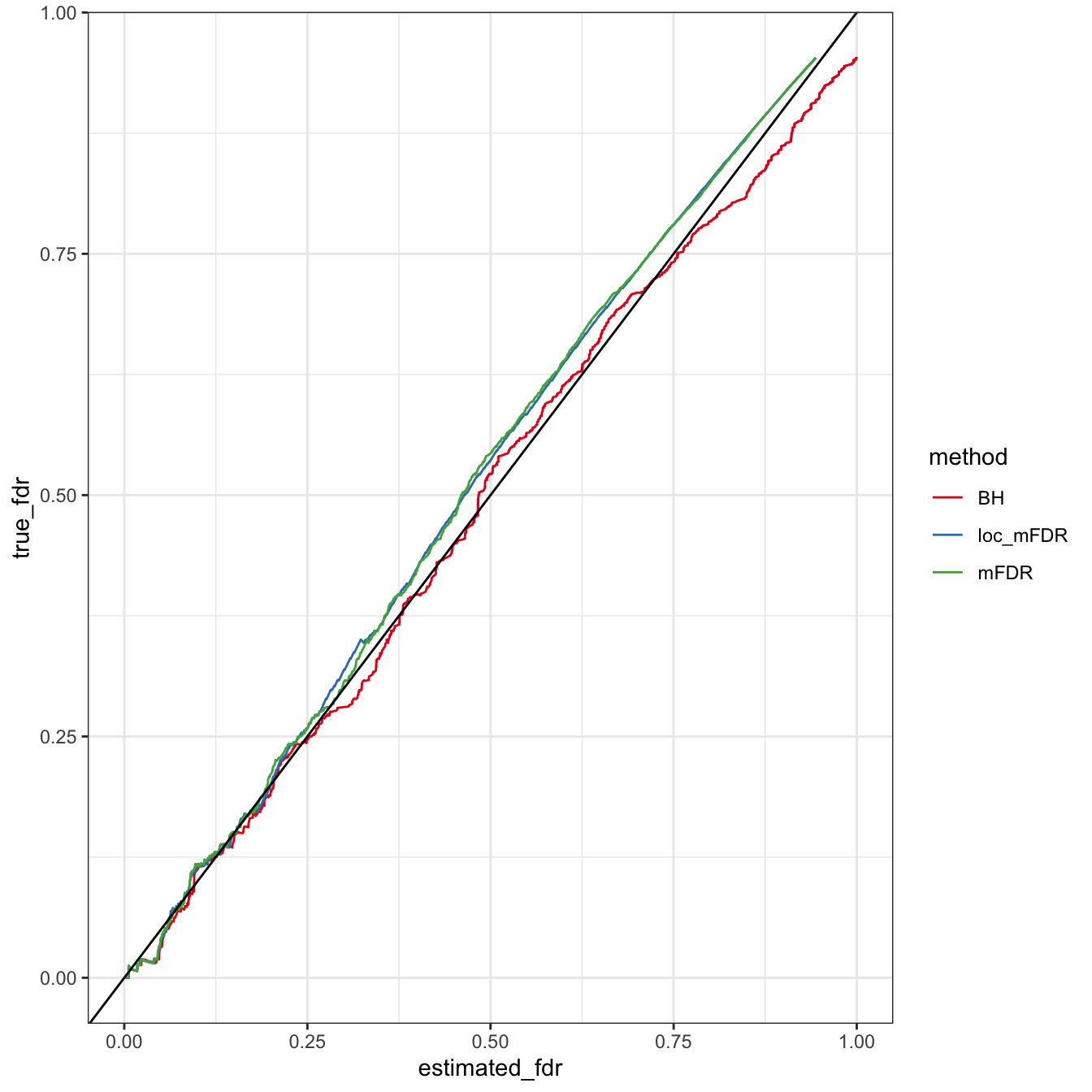

The empirical method is on-par with exact method, though the Benjamini-Hochberg FDRs show slightly better calibration with the true FDR.

Multi-dimensional case

Let’s now take a look at the hierarchical model. We’ll assume that each test/gene have 5 measurements, and the measurements for the non-null genes also follow a mixture distribution, e.g. \(f_{1} = (1 - q) f_{0} + q f_{2}\). This creates more uncertainty about the true positives.

set.seed(12345)
n_genes = 10000
n_guides_per_gene = 5
genes = rep(1:n_genes, each = n_guides_per_gene)
x = rep(0, times = length(genes))
mu0 = 0
mu1 = 2
sigma0 = 1
sigma1 = 1
p_gene = 0.9
p_guide = 0.5
gene_labels = rbinom(n_genes, prob = 1 - p_gene, 1)
for(i in 1:n_genes){
  if(gene_labels[i] == 0){
    x[which(genes == i)] = rnorm(n_guides_per_gene, mean = mu0, sd = sigma0)
  }
  else{
    # gene label == 1
    guide_labels = rbinom(n_guides_per_gene, prob = 1 - p_guide, 1)
    mu_vec = sapply(guide_labels, function(i) if(i == 1) mu1 else mu0)
    sigma_vec = sapply(guide_labels, function(i) if(i == 1) sigma1 else sigma0)
    x[which(genes == i)] = rnorm(n_guides_per_gene, mean = mu_vec, sd = sigma_vec)
  }
}

mixfit = mixtools::normalmixEM2comp(x, lambda = c(0.5, 0.5), 
                                    mu = c(0, 1), sigsqrd = c(1, 1))

## number of iterations= 1000

print("fitted proportions: ")

## [1] "fitted proportions: "

print(mixfit$lambda)

## [1] 0.8075129 0.1924871

print("fitted means: ")

## [1] "fitted means: "

print(mixfit$mu)

## [1] -0.05286371  0.72474277

print("fitted sd's: ")

## [1] "fitted sd's: "

print(mixfit$sigma)

## [1] 0.9720461 1.3047024

# taken from https://tinyheero.github.io/2015/10/13/mixture-model.html
plot_mix_comps <- function(x, mu, sigma, lam) {
  lam * dnorm(x, mu, sigma)
}
library(ggplot2)
ggplot(data.frame(x = x) ) +
  geom_histogram(aes(x, ..density..), binwidth = 1, colour = "black", 
                 fill = "white") +
  stat_function(geom = "line", fun = plot_mix_comps,
                args = list(mixfit$mu[1], mixfit$sigma[1], lam = mixfit$lambda[1]),
                colour = "red", lwd = 1.5) +
  stat_function(geom = "line", fun = plot_mix_comps,
                args = list(mixfit$mu[2], mixfit$sigma[2], lam = mixfit$lambda[2]),
                colour = "blue", lwd = 1.5) +
  ylab("Density") + theme_bw()

The hierarchical mixture model has likelihood (see the Methods section of https://link.springer.com/article/10.1186/s13059-018-1538-6) \[ \mathcal{L}(f_{0}, f_{1}, p, q | x_{1}, \ldots, x_{n}) = \prod_{g = 1}^{G} (1 - p) \prod_{i: g_{i} = g} f_{0} (x_{i}) + p \prod_{i : g_{i} = g} \big( (1 - q) f_{0} (x_{i}) + q f_{1} (x_{i}) \big). \] Because of the non-identifiability of \(p\) and \(q\) simultaneously, we marginalized over \(q\) (with a uniform prior) to obtain gene-level local false discovery rates \[ \text{locfdr}(g) = \int_{0}^{1} \frac{(\hat{\tau} / q) \prod_{i: g_{i} = g} q f_{1} (x_{i}) + (1 - q) f_{0} (x_{i}) }{(\hat{\tau} / q) \prod_{i: g_{i} = g} \big( q f_{1} (x_{i}) + (1 - q) f_{0} (x_{i}) \big) + (1 - \hat{\tau} / q) \prod_{i: g_{i} = g} f_{0} (x_{i})} d q. \] We then used the empirical FDR estimator to compute estimates for the global false discovery rates.

crisphiermixFit = CRISPhieRmix::CRISPhieRmix(x = x, geneIds = genes, 
                                             pq = 0.1, mu = 4, sigma = 1,
                                             nMesh = 100,  BIMODAL = FALSE,
                                             VERBOSE = TRUE, PLOT = TRUE,
                                             screenType = "GOF")

## no negative controls provided, fitting hierarchical normal model

## Loading required package: mixtools

## mixtools package, version 1.2.0, Released 2020-02-05
## This package is based upon work supported by the National Science Foundation under Grant No. SES-0518772.

## WARNING! NOT CONVERGENT! 
## number of iterations= 1000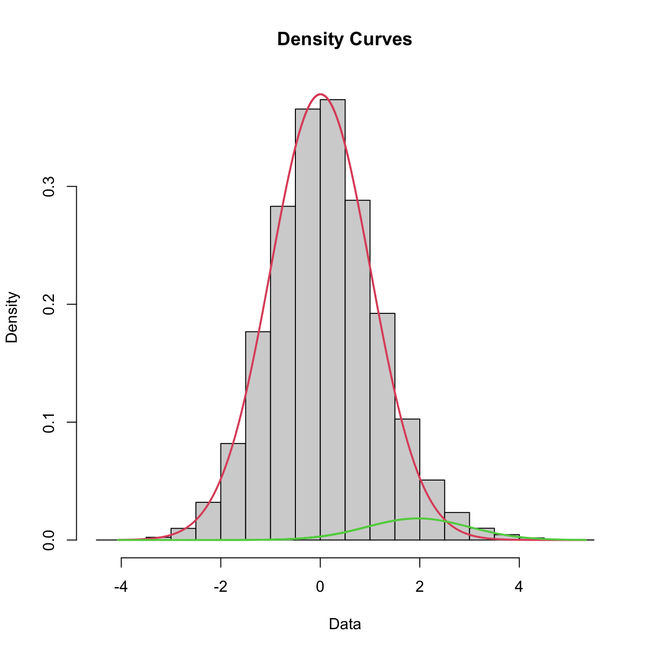

crisphiermixFit$mixFit$lambda

## [1] 0.95278182 0.04721818

crisphiermixFit$mixFit$mu

## [1] 0.004446553 1.960693489

crisphiermixFit$mixFit$sigma

## [1] 1.005094 1.028718

null_pvals = sapply(1:n_genes, function(g) t.test(x[which(genes == g)], alternative = "greater", mu = crisphiermixFit$mixFit$mu[1])$p.value)
bh_fdr = data.frame(estimated_FDR = p.adjust(null_pvals, method = "fdr"),
                    pvals = null_pvals)
bh_fdr['true_fdr'] = sapply(bh_fdr$estimated_FDR, function(p) sum(gene_labels[which(bh_fdr$estimated_FDR <= p)] == 0)/sum(bh_fdr$estimated_FDR <= p))
head(bh_fdr)

##   estimated_FDR     pvals  true_fdr
## 1     0.9795228 0.8252480 0.8871217
## 2     0.9390381 0.5319651 0.8395410
## 3     0.9797612 0.8294592 0.8880518
## 4     0.9857013 0.8827119 0.8933676
## 5     0.9470087 0.6006585 0.8558586
## 6     0.7356476 0.1166486 0.6505949

crisphiermixFDR = data.frame(estimated_FDR = crisphiermixFit$FDR)
crisphiermixFDR['true_fdr'] = sapply(crisphiermixFDR$estimated_FDR, function(p) sum(gene_labels[which(crisphiermixFDR$estimated_FDR <= p)] == 0)/sum(crisphiermixFDR$estimated_FDR <= p))
head(crisphiermixFDR)

##   estimated_FDR  true_fdr
## 1     0.8063019 0.8621093
## 2     0.8068114 0.8626709
## 3     0.8352201 0.8919991
## 4     0.8385534 0.8952391
## 5     0.7792940 0.8341960
## 6     0.6835582 0.7305573

cols = RColorBrewer::brewer.pal(8, 'Set1')
df = data.frame(estimated_FDR = c(crisphiermixFDR$estimated_FDR, bh_fdr$estimated_FDR),
                true_FDR = c(crisphiermixFDR$true_fdr, bh_fdr$true_fdr),
                method = rep(c("empirical FDR", "BH FDR"), each = dim(crisphiermixFDR)[1]))
ggplot(df, aes(y = true_FDR, x = estimated_FDR, col = method)) + geom_line() + theme_bw() + scale_colour_brewer(palette = "Set1") + geom_abline(intercept = 0, slope = 1)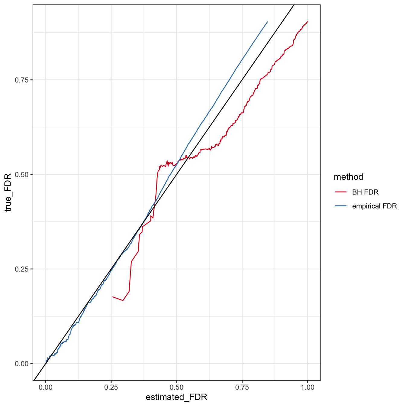

What’s happening with the Benjamini-Hochberg FDRs? Why aren’t many lower than 0.3?

head(bh_fdr[which(bh_fdr$estimated_FDR < 0.3), ])

##      estimated_FDR        pvals  true_fdr
## 20       0.2548441 0.0002241322 0.1764706
## 1069     0.2548441 0.0004236029 0.1764706
## 2342     0.2548441 0.0001856662 0.1764706
## 2750     0.2548441 0.0002576694 0.1764706
## 2897     0.2548441 0.0001255965 0.1764706
## 3433     0.2548441 0.0002680069 0.1764706

We see that the Benjamini-Hochberg-corrected \(t\)-test is not powerful enough to give meaningful insight into low false discovery rate region. Though, the rest of the region is well-calibrated. However, we see that the empirical estimator of the FDR is very well calibrated. At least in this case when the model is correctly specified. An argument could be made that the empirical estimator has the advantage of knowing the correct model, but that would lead the BH FDRs to not be calibrated and not what we see here.