Fisher vs Stouffer
Timothy Daley
11/29/2020
The most common way to coalesce \(p\)-values is Fisher’s method (https://en.wikipedia.org/wiki/Fisher%27s_method). The basic idea is to log transform your \(p\)-values, then \(-2\) times the sum is chi-square distributed. Specifically, for \(p\)-values \(p_{1}, \ldots, p_{n}\), Fisher’s method calculates the combined test statistic as \[ t_{\text{Fisher}} = -2 \sum_{i = 1}^{n} \log p_{i}. \] Under the null that the \(p\)-values are independent uniformly distributed, the test statistic \(t_{\text{Fisher}}\) will be \(\chi^{2}_{2n}\) distributed. The common wisdom is that Fisher’s method tend to values low p-values, instead of consistently low \(p\)-values.
An alternative to Fisher’s method is Stouffer’s method. The idea is to transform the \(p\)-values to \(z\)-scores, then compute a combined \(z\)-score by averaging the individual \(z\)-scores. E.g. if \(\Phi(\cdot)\) is the standard normal cdf, then the test statistic is \[ t_{\text{Stouffer}} = \frac{1}{\sqrt{k}} \sum_{i = 1}^{n} \Phi^{-1} (p_{i}). \] Under the null this is distributed as a negative standard normal variable (negative because \(\Phi^{-1}\) of small \(p\)-values will be less than zero). The prevailing wisdom is that this method values consistently small \(p\)-values. To ensure that effects have the same sign, we can define \[ t_{\text{Stouffer}} = \frac{1}{\sqrt{k}} \sum_{i = 1}^{n} \text{sign}(x_{i}) \Phi^{-1} (p_{i}) \] as the test statistic so that effect sizes (\(x_{i}\)) of the same sign are valued. This has a null distribution of standard normal.
I first learned about Stouffer’s method through a paper by Art Owen which discusses different meta-analysis techniques. In particular, he says “In the Fisher test, if the first \(m−1\) \(p\)-values already yield a test statistic exceeding the \(\chi^2_{2m}\) significance threshold, then the \(m\)th test statistic cannot undo it. The Stouffer test is different. Any large but finite value of \(\sum_{j = 1}^{m-1} \Phi^{-1}(p_{j})\) can be canceled by an opposing value of \(\Phi^{-1}(p_{m})\).” Thus indicating that Stouffer’s method will tend to pick up more small but consistent effects, and will be more robust in the presence of rare outliers. On the other hand, because Fisher’s method can be significant due to just one very small \(p\)-value then it is likely not as robust to outliers. To test this let’s compare the methods in two situations: small-tailed null and long-tailed null, where the latter will simulate the presence of outlier effects. I expect that Fisher’s method will have higher false positive in the presence of long tails.
Simulation
The simulation I’ll run is the standard 2-groups model (e.g. see Efron 2008). For aggregation purposes, we’ll have 5 effect sizes (I’m leaving effect size undefined on purpose) to merge. In the motivating application, the individual effect sizes and \(p\)-values arise from differential expression analysis of guide RNAs, with aggregation done at the gene level (as guide RNAs target specific genes). Consistent effects are not guaranteed because of variable guide efficiency (e.g. see my previous paper on this topic).
library(reticulate)
# you need to edit RETICULATE_PYTHON in .Renviron
# for some reason I need to make a venv for each project
Sys.setenv(RETICULATE_PYTHON = "/Users/tim.daley/blog/FisherVsStouffer/venv/bin/python3")
use_python('/Users/tim.daley/blog/FisherVsStouffer/venv/bin/python3')
#reticulate::py_config()
import numpy as np
# set seed
np.random.seed(12345)
n_genes = 20000
# 2% of genes are non-null
p = 0.05
gene_labels = np.random.binomial(n = 1, p = p, size = (n_genes, ))
print("number of genes: ", n_genes)## number of genes: 20000print("number of non-null genes: ", sum(gene_labels))## number of non-null genes: 1029Small tail
For the small-tailed case, let’s assume that null gene-effects are equal to \(0\) and the non-null gene effects are distributed \(\mathcal{N}(3, 1)\).
import seaborn
gene_effects = gene_labels*np.random.normal(loc = 3, scale = 1, size = (n_genes, ))
seaborn.histplot(gene_effects, color = 'black')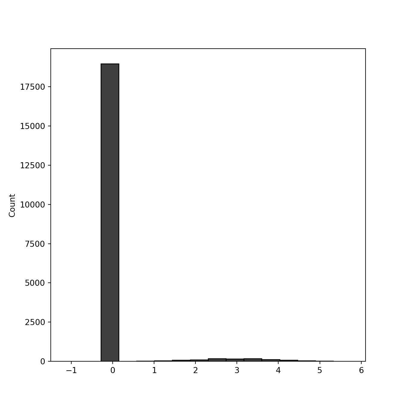
You can see the long tail on the right is the gene effects. Now let’s assume 5 observations (guide RNAs) per gene. These are gonna be normally distributed with mean equal to gene effect size, and standard deviation 1.
import itertools
import pandas as pd

lst = range(n_genes)
guide2gene_map = list(itertools.chain.from_iterable(itertools.repeat(x, 5) for x in lst))
n_guides = 5*n_genes
assert(len(guide2gene_map) == n_guides)

guide_effects = pd.DataFrame({'guide2gene': guide2gene_map})
guide_effects['guide_effect'] = guide_effects['guide2gene'].map(lambda i: np.random.normal(loc = gene_effects[i], scale = 1))
guide_effects['label'] = guide_effects['guide2gene'].map(lambda i: gene_labels[i])
seaborn.histplot(x = 'guide_effect', hue = 'label', data = guide_effects).set_title('guide effect distribution')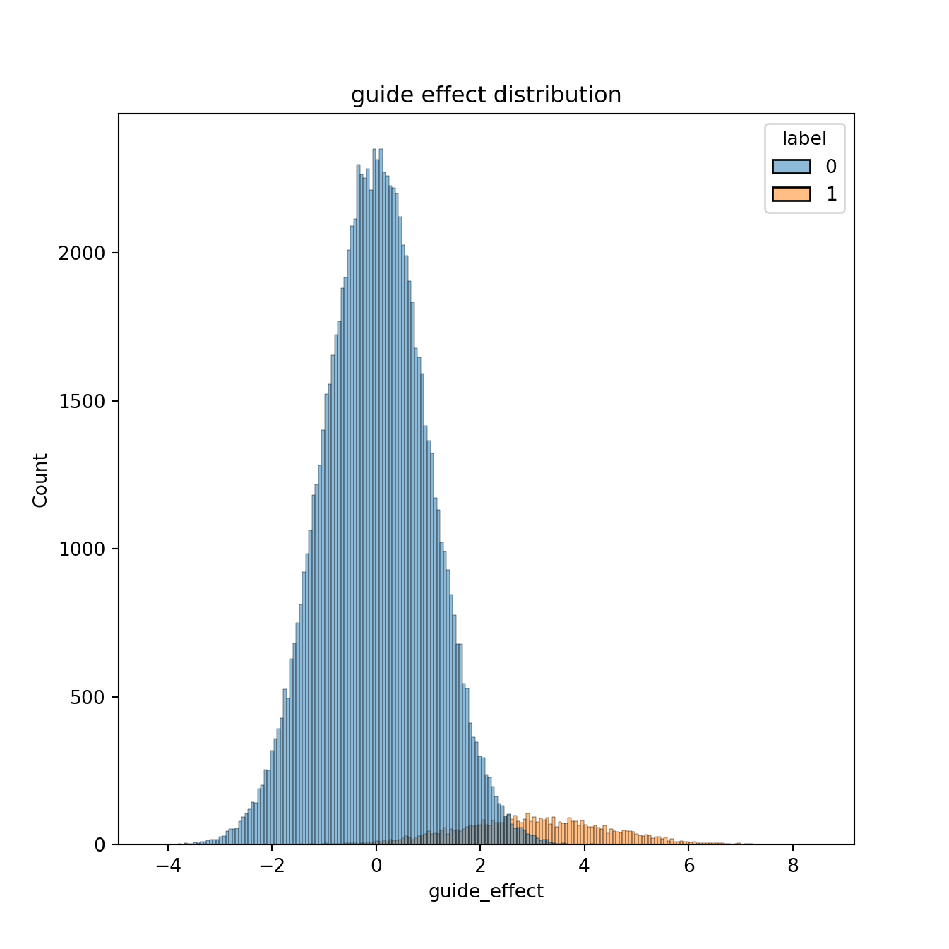
Now let’s look at combining \(p\)-values with Fisher vs Stouffer.
from scipy.stats import norm, chi2
from math import sqrt

def stouffer_pval(z):
  stouffer_zval = sum(z)/sqrt(len(z))
  stouffer_pval = norm.cdf(-stouffer_zval)
  return stouffer_pval

def fisher_pval(z):
  # 1-sided p-val
  pvals = norm.cdf(-z)
  fisher_val = -2*sum(np.log(pvals))
  fisher_pval = 1.0 - chi2.cdf(fisher_val, df = 2*len(z))
  return fisher_pval

gene_pvals = pd.DataFrame({'gene': range(n_genes),
                           'gene_label': gene_labels})

gene_pvals['fisher'] = gene_pvals['gene'].map(lambda i: fisher_pval(guide_effects[guide_effects['guide2gene'] == gene_pvals['gene'][i]]['guide_effect']))
gene_pvals['stouffer'] = gene_pvals['gene'].map(lambda i: stouffer_pval(guide_effects[guide_effects['guide2gene'] == gene_pvals['gene'][i]]['guide_effect']))

gene_pvals.head()
## gene gene_label fisher stouffer
## 0 0 0 0.620273 0.508737
## 1 1 0 0.873517 0.868306
## 2 2 0 0.509792 0.379961
## 3 3 0 0.372420 0.446334
## 4 4 0 0.398732 0.542383import matplotlib.pyplot as plt
seaborn.histplot(gene_pvals['fisher'], bins = 30, color = 'black', label = 'Fisher p-vals')
plt.show()
seaborn.histplot(gene_pvals['stouffer'], bins = 30, color = 'black', label = 'Stouffer p-vals')
plt.show()
Now let’s compute Benjamini-Hochberg FDRs and compare them to the empirical FDR.
from statsmodels.stats.multitest import fdrcorrection

_, gene_pvals['fisher_fdr'] = fdrcorrection(gene_pvals['fisher'], method = 'indep')

_, gene_pvals['stouffer_fdr'] = fdrcorrection(gene_pvals['stouffer'], method = 'indep')

gene_pvals.head()
## gene gene_label fisher stouffer fisher_fdr stouffer_fdr
## 0 0 0 0.620273 0.508737 0.970138 0.953773
## 1 1 0 0.873517 0.868306 0.990323 0.991374
## 2 2 0 0.509792 0.379961 0.956906 0.921007
## 3 3 0 0.372420 0.446334 0.920225 0.940338
## 4 4 0 0.398732 0.542383 0.926149 0.956265Now let’s compute the empirical FDRs.
def compute_empirical_fdr(labels, fdrs, fdr_thresh):
  mask = (fdrs < fdr_thresh)
  R = np.sum(mask)
  if R > 0:
    return np.sum(1 - labels[mask])/float(R)
  else:
    return 0

empirical_fdr = pd.DataFrame({'fdr_thresh': np.linspace(0, 1, num = 1000)})
empirical_fdr['fisher'] = empirical_fdr['fdr_thresh'].map(lambda x: compute_empirical_fdr(gene_pvals['gene_label'], gene_pvals['fisher_fdr'], x))

empirical_fdr['stouffer'] = empirical_fdr['fdr_thresh'].map(lambda x: compute_empirical_fdr(gene_pvals['gene_label'], gene_pvals['stouffer_fdr'], x))

empirical_fdr.head()
## fdr_thresh fisher stouffer
## 0 0.000000 0.000000 0.000000
## 1 0.001001 0.001147 0.001121
## 2 0.002002 0.002227 0.003293
## 3 0.003003 0.004410 0.004362
## 4 0.004004 0.007650 0.007559empirical_fdr.tail()## fdr_thresh fisher stouffer
## 995 0.995996 0.945746 0.945044
## 996 0.996997 0.946220 0.945427
## 997 0.997998 0.948362 0.947968
## 998 0.998999 0.948434 0.948398
## 999 1.000000 0.948550 0.948550df = pd.DataFrame({'estimated_fdr': empirical_fdr['fdr_thresh'].tolist() + empirical_fdr['fdr_thresh'].tolist(),
'empirical_fdr': empirical_fdr['fisher'].tolist() + empirical_fdr['stouffer'].tolist(),
'condition': ['fisher']*empirical_fdr.shape[0] + ['stouffer']*empirical_fdr.shape[0]})
plt.plot([0, 1], [0, 1], '--', color = 'black')## [<matplotlib.lines.Line2D object at 0x7ffd20a440d0>]seaborn.lineplot(x = 'estimated_fdr', y = 'empirical_fdr', hue = 'condition', data = df)## <AxesSubplot:xlabel='estimated_fdr', ylabel='empirical_fdr'>plt.show()
Long tail
Now what happens if the null is a long-tailed distribution? We’ll use a t-distribution with a finite variance as the long tailed, and we’ll normalize it so that the standard deviation is equal to 1.
import pandas as pd
from math import sqrt
long_tailed_guide_effects = pd.DataFrame({'guide2gene': guide2gene_map})
deg_fred = 5
sd = sqrt(deg_fred/float(deg_fred - 2))
# divide by sd to normalize
long_tailed_guide_effects['guide_effect'] = long_tailed_guide_effects['guide2gene'].map(lambda i: gene_effects[i] + np.random.standard_t(df = deg_fred)/sd)
long_tailed_guide_effects['label'] = long_tailed_guide_effects['guide2gene'].map(lambda i: gene_labels[i])
seaborn.histplot(x = 'guide_effect', hue = 'label', data = long_tailed_guide_effects)
## <AxesSubplot:xlabel='guide_effect', ylabel='Count'>plt.show()
long_tailed_gene_pvals = pd.DataFrame({'gene': range(n_genes),
                           'gene_label': gene_labels})

long_tailed_gene_pvals['fisher'] = long_tailed_gene_pvals['gene'].map(lambda i: fisher_pval(long_tailed_guide_effects[long_tailed_guide_effects['guide2gene'] == long_tailed_gene_pvals['gene'][i]]['guide_effect']))
long_tailed_gene_pvals['stouffer'] = long_tailed_gene_pvals['gene'].map(lambda i: stouffer_pval(long_tailed_guide_effects[long_tailed_guide_effects['guide2gene'] == long_tailed_gene_pvals['gene'][i]]['guide_effect']))
_, long_tailed_gene_pvals['fisher_fdr'] = fdrcorrection(long_tailed_gene_pvals['fisher'], method = 'indep')

_, long_tailed_gene_pvals['stouffer_fdr'] = fdrcorrection(long_tailed_gene_pvals['stouffer'], method = 'indep')

long_tailed_empirical_fdr = pd.DataFrame({'fdr_thresh': np.linspace(0, 1, num = 1000)})
long_tailed_empirical_fdr['fisher'] = long_tailed_empirical_fdr['fdr_thresh'].map(lambda x: compute_empirical_fdr(long_tailed_gene_pvals['gene_label'], long_tailed_gene_pvals['fisher_fdr'], x))
long_tailed_empirical_fdr['stouffer'] = long_tailed_empirical_fdr['fdr_thresh'].map(lambda x: compute_empirical_fdr(long_tailed_gene_pvals['gene_label'], long_tailed_gene_pvals['stouffer_fdr'], x))

df = pd.DataFrame({'estimated_fdr': long_tailed_empirical_fdr['fdr_thresh'].tolist() + long_tailed_empirical_fdr['fdr_thresh'].tolist(),
                   'empirical_fdr': long_tailed_empirical_fdr['fisher'].tolist() + long_tailed_empirical_fdr['stouffer'].tolist(),
                   'condition': ['fisher']*long_tailed_empirical_fdr.shape[0] + ['stouffer']*long_tailed_empirical_fdr.shape[0]})
plt.plot([0, 1], [0, 1], '--', color = 'black')## [<matplotlib.lines.Line2D object at 0x7ffd1083e070>]seaborn.lineplot(x = 'estimated_fdr', y = 'empirical_fdr', hue = 'condition', data = df)## <AxesSubplot:xlabel='estimated_fdr', ylabel='empirical_fdr'>plt.show()
We see here that Fisher’s method has a higher false positive rate, particularly in the lower region where we usually set the false discovery rate. This inidicates that Fisher’s method is much more susceptible to false positives in the presence of long tails. If we correctly specify the null model, then this will be less of an issue, but we saw above that both methods perform similarly when the model is correctly specified. Therefore, this simple experiment indicates that there can be significant benefits to using Stouffer’s method in place of Fisher’s method, particularly when long-tailed or off-target effects can be present in the null distribution and are difficult to accurately model.